Introduction
The main objective of our recommender systems is to narrow down Wayfair’s vast catalogue to assist customers in finding exactly the products they want. Most recommendation algorithms leverage a customer’s browsing history, which includes various types of interactions with products, such as clicks, add-to-cart actions, and orders. The diversity of each customer’s browsing history makes the task of fully leveraging the information it contains quite difficult. One of the challenges with a diverse browsing history is determining whether we can use a customer’s interactions with products in one category to recommend relevant products in another category. For example, if a customer has browsed beds and dressers, we would like to recommend items in a complementary class—like nightstands—as well. Such recommendations would allow a customer to find useful products that fit her style before she begins to wade through the potentially overwhelming options in that category. Being able to help customers find items from classes of furniture that they have not browsed, interacted with, or searched for, would therefore significantly improve the online shopping experience.
Applying standard Collaborative Filtering techniques in a cross-category scenario like the one mentioned above is challenging. First off, approaches based on similarity indices like the Jaccard Index are computationally expensive. To compute similarity indices in a cross-class recommendation scenario, we need to compute customer interactions between millions of products from thousands of categories. Additionally, a pairwise computation is not scalable or maintainable when categories are updated and expanded frequently. Also, matrix factorization methods applied on large and sparse matrices encoding browsing history on large categories takes time to converge, and can be numerically unstable. Considering these obstacles, we on the Data Science Product Recommendations team decided to explore alternative approaches.
In this post, we’ll be walking through one of the exciting approaches we've developed here at Wayfair, ReCNet (Really Cool Network), a deep-learning-based hybrid recommendation model, framed as a metric learning problem. ReCNet supports complementary recommendations across the Wayfair catalogue, and is actively being expanded to many use cases.
Method
To apply deep learning techniques in a real world business, one must consider four critical components: problem transformation, model architecture, loss function design, and production deployment. We will cover each of these in the following sections.
Problem Transformation: Metric Learning
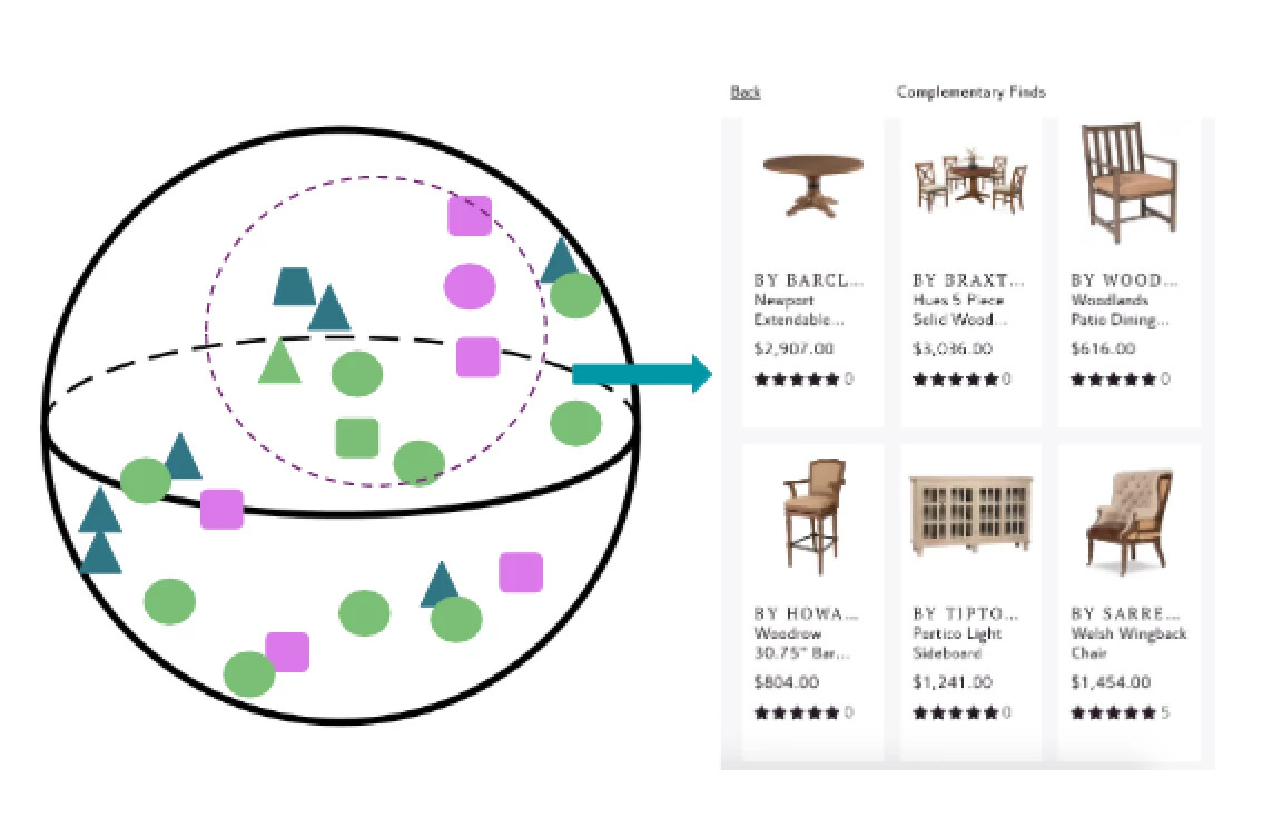
Intuitively, in a cross-category scenario, a product is recommended to a customer because it goes well with a product from another category owned or browsed by this customer. Imagine there exists such a space where products that go well together are close to each other. Then in this space, the distance between two products actually measures how closely matched they are, which is the main goal of tackling cross-class recommendations as a metric learning problem. In metric learning, a model is trained to create a latent space encoding properties contained within the learned metric. For instance, in the work of FaceNet, Euclidean distance in the latent space measures facial similarity [1]. Metric learning is also applied in the fashion industry to learn clothing style [2], where vector representations of stylistically similar clothing are close to each other in the space. In our use case, products that are frequently purchased, added to user-curated idea boards together, or that share the same style tag will be close to each other in the metric space. We define these products as being stylistically similar. Additionally, products which have similar side information (price, ratings, review counts, etc.) will be even closer. The problem then becomes how to create such a space.

Model Architecture: Siamese Network
In our ReCNet model, we train a siamese network where each leg is multimodal and uses a wide-and-deep architecture [3]. The input to the siamese network is a pair of product images and their side information vectors. Each leg in the siamese network has a wide subnetwork and a deep subnetwork.

Google’s team developed the deep subnetwork to generalize and the wide subnetwork to memorize [3]. We made some modifications to this framework to favor our use case, training a shallow network as the wide subnetwork to learn a vector representation from side information. We perform transfer learning from one version of Wayfair’s in-house Visual Search model to initialize the deep subnetwork, based on the Inception V3 architecture. Through the deep subnetwork, an embedding vector (I) derived from image features is learned. Meanwhile, the wide subnetwork learns an embedding vector (S) from side information features. The side information features are fed into a one-layer wide subnetwork to memorize slightly abstracted features, aimed at preventing the network from over-fitting, while still converging to better local optimum. Then, a synthetic embedding for each product is generated by concatenating I and S and performing L2-normalization on the resulting vector. In this way, the synthetic embeddings are located on a unit hypersphere and have image information represented in some dimensions and side information encoded in the others.
Loss Function Design: Customized Constrastive Loss
Even with the synthetic embeddings, we still need a loss function to train the model. The original contrastive loss function injects loss when two items in a matching pair are far away from each other or two items in a non-matching pair are too close within a certain margin in the metric space [4]. The original loss function is defined as

where Y is a binary label of whether two products are stylistically similar or not. Dw is the distance metric between X1 and X2, the two learned product vectors. M measures the margin that products must exhibit if they do not match. In other words, it’s the minimum distance needed between them to not impose loss. On top of that, we incorporate the notion of image information embedding dimensions (I) and side information embedding dimensions (S) in

Where

Here y labels whether two products are similar according to side information and m measures the size of the margin dissimilar products should be from one another in the learned space. Alpha is the weight for side information relative to image information. In general, the customized loss function can be viewed as two nested contrastive loss functions applied on side information dimensions and image information dimensions. Given two labels, Y and y, the customized loss function can be broken down into four cases:
1. If two products are stylistically similar (Y = 1) and have similar side information (y = 1), loss is introduced if they are too far away in image embedding dimensions and side information embedding dimensions.

2. If two products are not stylistically similar (Y = 0) but share similar side information (y = 1), loss is introduced if they are too close in image embedding dimensions.

3. If two products are stylistically similar (Y = 1) but are not similar in side information (y = 0), loss is introduced if they are too far away in image embedding dimensions and too close in side information embedding dimensions.

4. If two products are not stylistically similar (Y = 0) neither are they similar in side information (y = 0), loss is introduced if they are too close in image embedding dimensions.

Production Deployment: Nearest Neighbors as Recommendations
Once the model architecture has been determined, we apply stochastic gradient descent with a cyclic learning rate to train the model [5]. We then load one leg from the siamese network into memory, and use it to embed all products from the catalog. The embeddings are vector representations of the products in ReCNet latent space. To generate recommendations, we just need to query the nearest neighbors of the products in a customer’s browsing history. To do this, we use data structures designed for a fast and efficient nearest neighbor search. Deterministic data structures—like ball trees—can be used to solve this kind of problem, as well as probabilistic data structures like hierarchical navigable small world graphs. These latter structures improve upon the performance of ball trees, but provide an approximate nearest neighbor search, rather than an exact one. We find that hierarchical navigable small world graphs work quite well in production and generate reasonable results as in the following section.
Results
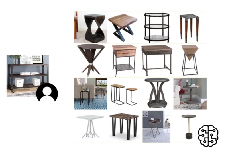
The following is a qualitative example of leveraging a console table to generate end table recommendations. We see here the wooden glossy console table has classic, but simple design. ReCNet is able to capture the design and find stylistically similar end tables as recommendations with diversity in shape and structure. Since the model learns from product images and side information, it has a content-based property which prevents us from suffering from the cold start problem. Also due to the content-based property, ReCNet digs deeper into the catalog to expose more stylistically similar products to customers.

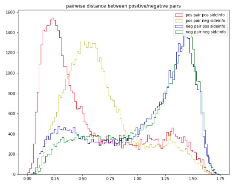
Now we have a sense of how the model is working qualitatively. But how is it functioning from a quantitative perspective? Is the model really learning a latent space as expected or reflected in the customized loss function? Upon further inspection of the latent space, we pull product pairs from our testing set, and compute the pairwise distances between them. The distribution of these distances can be seen in this plot with different colors indicating each one of the four label combinations.


The trimodal distribution confirms that ReCNet is capable of fine tuning the metric based on side information. The majority of the products that are stylistically similar and match in side information (red) are closer to each other than the products that are stylistically similar, but not similar in side information (yellow). Products that are not stylistically similar, regardless of if they are similar in side information, are further away. Overlap between the blue and green distribution is expected since we don’t distinguish whether the products share similar side information as long as they aren’t stylistically similar. In this way, when we do a nearest neighbor search in this latent space, we retrieve not only the most stylistically similar results, but also ones that match along dimensions of side information such as price, rating, etc.
Future Work
In the future, we will look to implement a triplet loss with the notion of two different margins/labels creating four possible combinations of label configurations. In addition, we will look to insert ReCNet into the current personalization framework to support recommendations in other use cases like online ads and marketing emails. Wayfair Data Science is never done, so stay tuned for more updates on the Wayfair tech blog!
References
[1] Schroff, F., Kalenichenko, D., & Philbin, J. (2015). FaceNet: A unified embedding for face recognition and clustering. 2015 IEEE Conference on Computer Vision and Pattern Recognition (CVPR). doi: 10.1109/cvpr.2015.7298682. P. 5
[2] Veit, A., Kovacs, B., Bell, S., Mcauley, J., Bala, K., & Belongie, S. (2015). Learning Visual Clothing Style with Heterogeneous Dyadic Co-Occurrences. 2015 IEEE International Conference on Computer Vision (ICCV). doi: 10.1109/iccv.2015.527. P. 3
[3] Cheng, H.-T., Ispir, M., Anil, R., Haque, Z., Hong, L., Jain, V., … Chai, W. (2016). Wide & Deep Learning for Recommender Systems. Proceedings of the 1st Workshop on Deep Learning for Recommender Systems - DLRS 2016. doi: 10.1145/2988450.2988454. P. 30
[4] Hadsell, R., Chopra, S., & Lecun, Y. (n.d.). Dimensionality Reduction by Learning an Invariant Mapping. 2006 IEEE Computer Society Conference on Computer Vision and Pattern Recognition - Volume 2 (CVPR06). doi: 10.1109/cvpr.2006.100. P. 16
[5] Smith, L. N. (2017). Cyclical Learning Rates for Training Neural Networks. 2017 IEEE Winter Conference on Applications of Computer Vision (WACV). doi: 10.1109/wacv.2017.58. P. 4

